Differential Expression using Rstudio

Approximate time: 60 minutes

Learning Objectives

• Use R to perform differential expression analysis

Step 1. Setup Rstudio on the Tufts HPC cluster via “On Demand”

1. Open a Chrome browser and visit ondemand.cluster.tufts.edu
2. Log in with your Tufts Credentials
3. On the top menu bar choose Interactive Apps -> Rstudio
4. Choose:

Number of hours  : 4
Number of cores  : 1
Amount of Memory : 32 Gb
R version        : 3.5.0
Partition        : Default
Reservation      : Default

Note if you are registered for the workshop, you may instead choose the following options in order to take advantage of a reservation that will be available for one week after the workshop start date:

Partition        : Preempt
Reservation      : Bioworkshop

Step 2. Working with Rstudio Interface

Go to the File menu -> New File -> R Script, you should see:

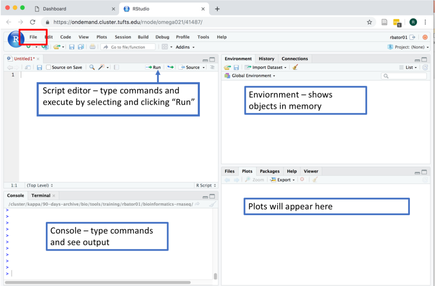
To save current session, click: File menu -> Save your file as intro.R

• Set up working directory and library

To run the code in the script editor, select a single line of code or highlight a block of code and click “Run”. To see your current working directory:

getwd()

To change to our workshop directory:

setwd('/cluster/tufts/bio/tools/training/intro-to-rnaseq/users/YOUR_USERNAME/into-to-RNA-seq/')

Check which paths on the cluster R will use to find library locations:

.libPaths()

Since we will be using a lot of R libraries today for differential expression analysis, instead of installing these libraries, you can use common library from Tufts bio tools by running:

.libPaths('/cluster/tufts/bio/tools/R_libs/3.5')

Now, you will be able to use all the libraries needed for this course. To load a library, type:

library(tidyverse)

• Read in Data

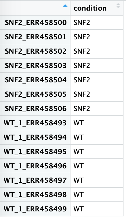
To read in the metadata for our experiment:

meta <- read.table("./raw_data/sample_info.txt", header=TRUE)

You can view the data by typing meta or view(meta)

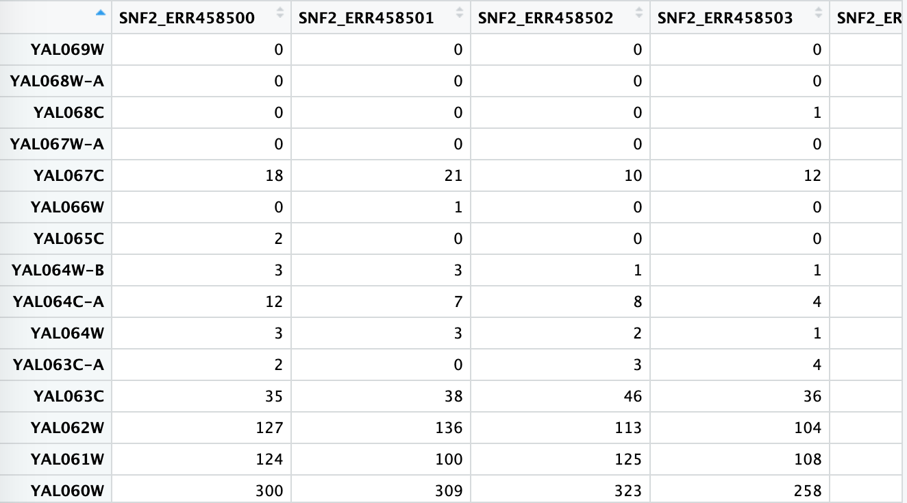
Load preprocessed data set of 7 WT replicates and 7 SNF2 knockouts

feature_count <- read.table("./featurecounts/featurecounts_results.mod.txt",
                            header=TRUE, row.names = 1)
# First 6 columns contain information about the transcripts. Here we only need the feature count informat. So we will remove first 6 columns by select the column 6 to 19
data <- feature_count[,6:19]
view(data)

Similarly, you can view the data by typing data or view(data)

DESeq2: Create DESeq2 Dataset object

Before running DESeq2, load all required libraries by running below:

# Put HPC biotools R libraries on your R path
.libPaths(c('', '/cluster/tufts/bio/tools/R_libs/3.5/'))
# load required libraries
library(DESeq2)
library(vsn)
library(dplyr)
library(tidyverse)
library(ggrepel)
library(DEGreport)
library(pheatmap)

To run DESeq2 analysis, you have to check to make sure that all rows labels in meta are columns in data:

all(colnames(data) == rownames(meta))

Create the dataset and run the analysis:

dds <- DESeqDataSetFromMatrix(countData = data, colData = meta, design = ~ condition)
dds <- DESeq(dds)

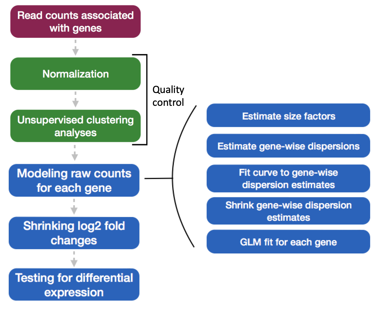
Behind the scenes these steps were run: 1.estimating size factors 2.gene-wise dispersion estimates 3.mean-dispersion relationship 4.final dispersion estimates 5.fitting model and testing

The design formula design = ~condition tells DESeq2 which factors in the metadata to test, such as control v.s. treatment. Here our condition is WT v.s. SNF2 as shown in the meta. The design can include multiple factors that are columns in the metadata. In this case, the factor that you are testing for comes last, and factors that you want to account for come first. E.g. To test for differences in condition while accounting for sex and age: design = ~ sex + age + condition. It’s also possible to include time series data and interactions.

• Normalization

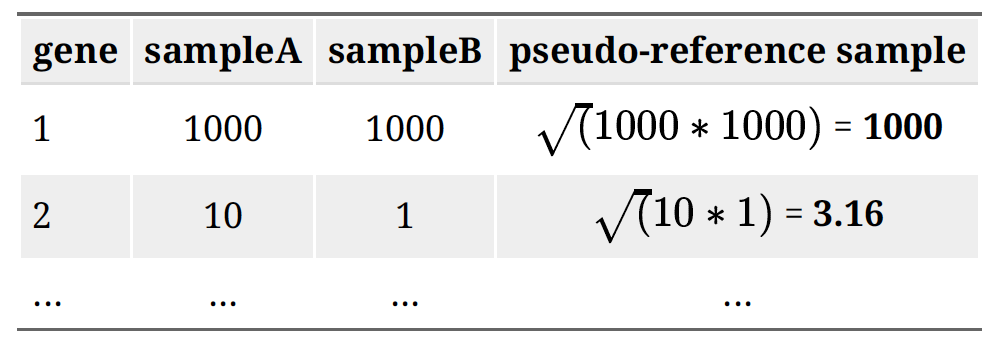
The number of sequenced reads mapped to a gene depends on: Gene Length, Sequencing depth, The expression level of other genes in the sample and Its own expression level. Normalization using DESeq2 accounts for both sequencing depth and composition. Step 1: creates a pseudo-reference sample (row-wise geometric mean). For each gene, a pseudo-reference sample is created that is equal to the geometric mean across all samples.

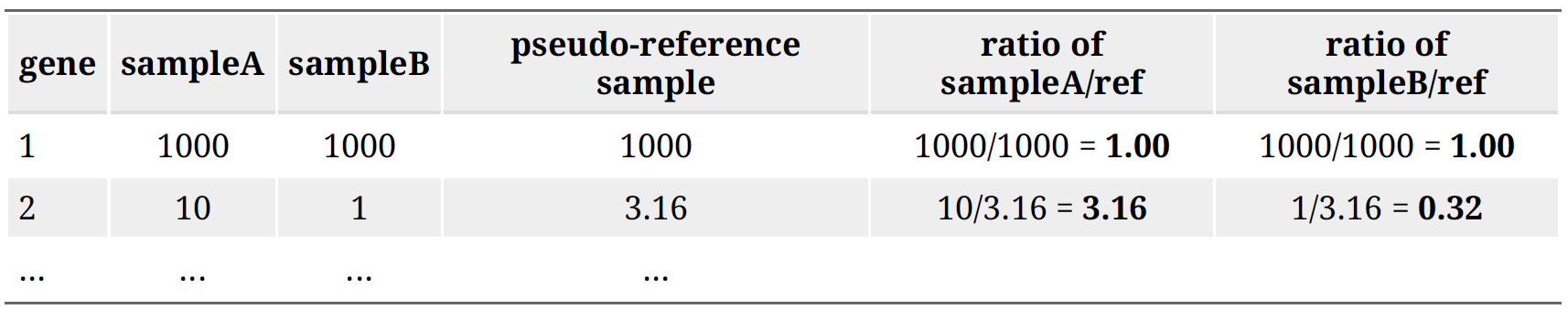
Step 2: calculates ratio of each sample to the reference. Calculate the ratio of each sample to the pseudo-reference. Since most genes aren’t differentially expressed, ratios should be similar.

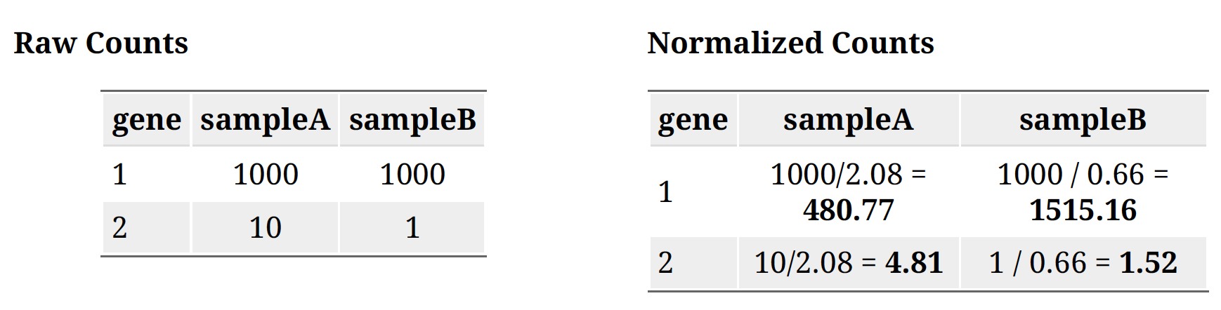
Step 3: calculate the normalization factor for each sample (size factor). The median value of all ratios for a given sample is taken as the normalization factor (size factor) for that sample:

normalization_factor_sampleA <- median(c(1.00, 3.16)) = 2.08
normalization_factor_sampleB <- median(c(1.00, 0.32)) = 0.66

Step 4: calculate the normalized count values using the normalization factor. This is performed by dividing each raw count value in a given sample by that sample’s size factor to generate normalized count values.

SampleA normalization factor = 2.08
SampleB normalization factor = 0.66

• Unsupervised Clustering

This step is to asses overall similarity between samples: 1.Which samples are similar to each other, which are different? 2.Does this fit to the expectation from the experiment’s design? 3.What are the major sources of variation in the dataset?

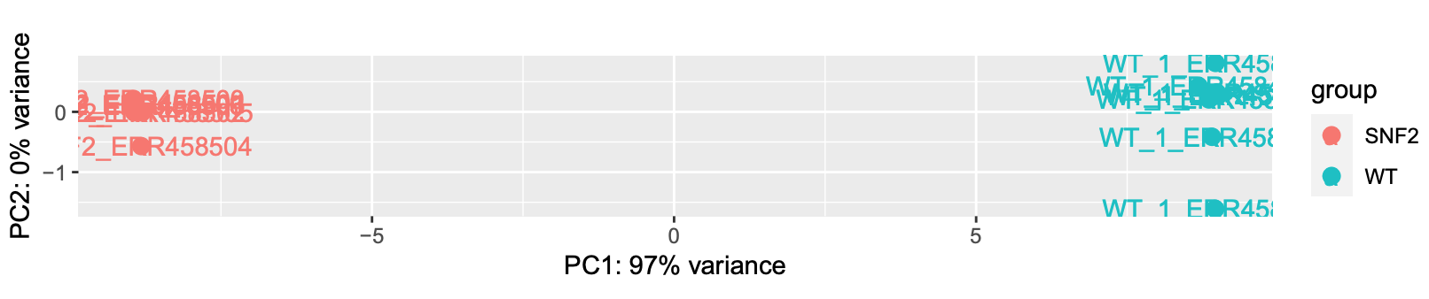
• Principle Components Analysis

This uses the built in function plotPCA from DESeq2 (built on top of ggplot). The regularized log transform (rlog) improves clustering by log transforming the data.

rld <- rlog(dds, blind=TRUE)
plotPCA(rld, intgroup="condition") + geom_text(aes(label=name))

• Creating contrasts and running a Wald test

The null hypothesis: log fold change = 0 for across conditions. P-values are the probability of rejecting the null hypothesis for a given gene, and adjusted p values take into account that we’ve made many comparisons:

contrast <- c("condition", "SNF2", "WT")
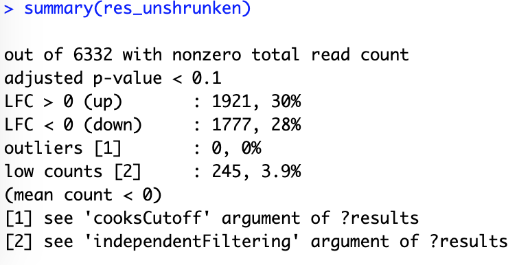
res_unshrunken <- results(dds, contrast=contrast)
summary(res_unshrunken)

Here shows a summary of up- or down-regulated genes:

• Shrinkage of the log2 fold changes

One more step where information is used across genes to avoid overestimates of differences between genes with high dispersion. This is not done by default, so we run the code:

res <- lfcShrink(dds, contrast=contrast, res=res_unshrunken)

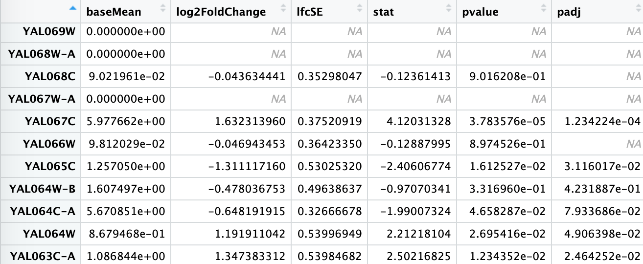
• Exploring results

The summary of results after shrinkage can be viewed by typing summary(res) or head(res). If you used head(res) you will be viewing the top few lines of the result containing log2 fold change and p-value. log2FoldChange = log2(SNF2count/WTcount)Estimated from the model. padj - Adjusted pvalue for the probability that the log2FoldChange is not zero.

1. Plot single gene Now, you can explore individual genes that you might be interested in. A simple plot can be made to compare the expression level of a particular gene. For example, for gene “YOR290C”:

   plotCounts(dds, gene="YOR290C", intgroup="condition")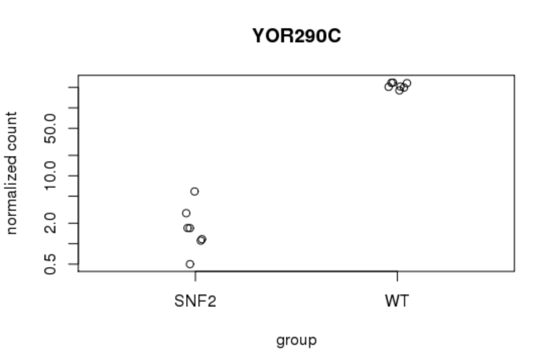
   

   

2. Saving the result Now you have the table with log2 fold change and you might want to save it for future analysis. A adj value cutoff can be applied here. For example, here p-adj 0.05 is used.

## Filtering to find significant genes
padj.cutoff <- 0.05 # False Discovery Rate cutoff
significant_results <- res[which(res$padj < padj.cutoff),]

## save results using customized file_name
file_name = 'significant_padj_0.05.txt'
write.table(significant_results, file_name, quote=FALSE)

Now you have your analyzed result saved in txt file, which can be imported to Excel.

• Exit R and save the work space

If you want to take a break and exit R, type q(). The workspace will be automatically saved with the extension of .Rproj.

Review DeSeq2 workflow

These comprise the full workflow

# Setup DESeq2
dds <- DESeqDataSetFromMatrix(countData = data, colData = meta, design = ~ condition)
# Run size factor estimation, dispersion estimation, dispersion shrinking, testing
dds <- DESeq(dds)
# Tell DESeq2 which conditions you would like to output
contrast <- c("condition", "SNF2", "WT")
# Output results to table
res_unshrunken <- results(dds, contrast=contrast)
# Shrink log fold changes for genes with high dispersion
res <- lfcShrink(dds, contrast=contrast, res=res_unshrunken)
# Regularized log transformation (rlog)
rld <- rlog(dds, blind=TRUE)

Workshop Schedule

• Course Home
• Introduction
• Setup using Tufts HPC
• Process Raw Reads
• Read Alignment
• Gene Quantification
• Currently at: Differential Expression
• Next: Pathway Enrichment